Comparing Means of Two Continuous Variables

Elements of a Designed Study

The problem of comparing more than two means results from the increase in Type I error that occurs when statistical tests are used repeatedly.

Learning Objectives

Discuss the increasing Type I error that accompanies comparisons of more than two means and the various methods of correcting this error.

Key Takeaways

KEY POINTS

• Unless the tests are perfectly dependent, the familywide error rate increases as the number of comparisons increases.
• Multiple testing correction refers to re-calculating probabilities obtained from a statistical test which was repeated multiple times.
• In order to retain a prescribed familywise error rate

  $\alpha$

  in an analysis involving more than one comparison, the error rate for each comparison must be more stringent than

  $\alpha$

  .
• The most conservative, but free of independency and distribution assumptions method, way of controlling the familywise error rate is known as the Bonferroni correction.
• Multiple comparison procedures are commonly used in an analysis of variance after obtaining a significant omnibus test result, like the ANOVA

  $\text{F}$

  -test.

KEY TERMS

• ANOVA: Analysis of variance—a collection of statistical models used to analyze the differences between group means and their associated procedures (such as "variation" among and between groups).
• Boole's inequality: a probability theory stating that for any finite or countable set of events, the probability that at least one of the events happens is no greater than the sum of the probabilities of the individual events
• Bonferroni correction: a method used to counteract the problem of multiple comparisons; considered the simplest and most conservative method to control the familywise error rate

For hypothesis testing, the problem of comparing more than two means results from the increase in Type I error that occurs when statistical tests are used repeatedly. If n independent comparisons are performed, the experiment-wide significance level

$\bar{\alpha}$

, also termed FWER for familywise error rate, is given by:

$\bar{\alpha}=1-(1-\alpha_\text{per comparison})^\text{n}$

Hence, unless the tests are perfectly dependent,

$\bar{\alpha}$

increases as the number of comparisons increases. If we do not assume that the comparisons are independent, then we can still say:

$\bar{\alpha}\leq{n}\cdot\alpha_\text{per comparison}$

There are different ways to assure that the familywise error rate is at most

$\bar{\alpha}$

. The most conservative, but free of independency and distribution assumptions method, is known as the Bonferroni correction

$\alpha_\text{per comparison}=\frac{\bar{\alpha}}{n}$

. A more sensitive correction can be obtained by solving the equation for the familywise error rate of independent comparisons for

$\alpha_\text{per comparison}$

.

This yields

$\alpha_\text{per comparison}=1-(1-\bar{\alpha})^\frac{1}{n}$

, which is known as the Šidák correction. Another procedure is the Holm–Bonferroni method, which uniformly delivers more power than the simple Bonferroni correction by testing only the most extreme

$\text{p}$

-value (

$\text{i}=1$

) against the strictest criterion, and the others (

$\text{i}>1$

) against progressively less strict criteria.

Methods

Multiple testing correction refers to re-calculating probabilities obtained from a statistical test which was repeated multiple times. In order to retain a prescribed familywise error rate

$\alpha$

in an analysis involving more than one comparison, the error rate for each comparison must be more stringent than

$\alpha$

. Boole's inequality implies that if each test is performed to have type I error rate αn, the total error rate will not exceed

$\alpha$

. This is called the Bonferroni correction and is one of the most commonly used approaches for multiple comparisons.

Because simple techniques such as the Bonferroni method can be too conservative, there has been a great deal of attention paid to developing better techniques, such that the overall rate of false positives can be maintained without inflating the rate of false negatives unnecessarily. Such methods can be divided into general categories:

• Methods where total alpha can be proved to never exceed 0.05 (or some other chosen value) under any conditions. These methods provide "strong" control against Type I error, in all conditions including a partially correct null hypothesis.
• Methods where total alpha can be proved not to exceed 0.05 except under certain defined conditions.
• Methods which rely on an omnibus test before proceeding to multiple comparisons. Typically these methods require a significant ANOVA/Tukey's range test before proceeding to multiple comparisons. These methods have "weak" control of Type I error.
• Empirical methods, which control the proportion of Type I errors adaptively, utilizing correlation and distribution characteristics of the observed data.

Post-Hoc Testing of ANOVA

Multiple comparison procedures are commonly used in an analysis of variance after obtaining a significant omnibus test result, like the ANOVA

$\text{F}$

-test. The significant ANOVA result suggests rejecting the global null hypothesis

$\text{H}_0$

that the means are the same across the groups being compared. Multiple comparison procedures are then used to determine which means differ. In a one-way ANOVA involving

$\text{K}$

group means, there are

$\frac{\text{K}(\text{K}-1)}{2}$

pairwise comparisons.

Randomized Design: Single-Factor

Completely randomized designs study the effects of one primary factor without the need to take other nuisance variables into account.

Learning Objectives

Discover how randomized experimental design allows researchers to study the effects of a single factor without taking into account other nuisance variables.

Key Takeaways

KEY POINTS

• In complete random design, the run sequence of the experimental units is determined randomly.
• The levels of the primary factor are also randomly assigned to the experimental units in complete random design.
• All completely randomized designs with one primary factor are defined by three numbers:

  $\text{k}$

  (the number of factors, which is always 1 for these designs),

  $\text{L}$

  (the number of levels), and

  $\text{n}$

  (the number of replications). The total sample size (number of runs) is

  $\text{N}=\text{k}\cdot\text{L}\cdot\text{n}$

  .

KEY TERMS

• factor: The explanatory, or independent, variable in an experiment.
• level: The specific value of a factor in an experiment.

In the design of experiments, completely randomized designs are for studying the effects of one primary factor without the need to take into account other nuisance variables. The experiment under a completely randomized design compares the values of a response variable based on the different levels of that primary factor. For completely randomized designs, the levels of the primary factor are randomly assigned to the experimental units.

Randomization

In complete random design, the run sequence of the experimental units is determined randomly. For example, if there are

$3$

levels of the primary factor with each level to be run

$2$

times, then there are

$6!$

(where "

$!$

" denotes factorial) possible run sequences (or ways to order the experimental trials). Because of the replication, the number of unique orderings is

$90$

(since

$90=6!2!2!2!$

). An example of an unrandomized design would be to always run

$2$

replications for the first level, then

$2$

for the second level, and finally

$2$

for the third level. To randomize the runs, one way would be to put

$6$

slips of paper in a box with

$2$

having level

$1$

,

$2$

having level

$2$

, and

$2$

having level

$3$

. Before each run, one of the slips would be drawn blindly from the box and the level selected would be used for the next run of the experiment.

Three Key Numbers

All completely randomized designs with one primary factor are defined by three numbers:

$\text{k}$

(the number of factors, which is always

$1$

for these designs),

$\text{L}$

(the number of levels), and

$\text{n}$

(the number of replications). The total sample size (number of runs) is

$\text{N}=\text{k}\cdot\text{L}\cdot\text{n}$

. Balance dictates that the number of replications be the same at each level of the factor (this will maximize the sensitivity of subsequent statistical

$\text{t}$

- (or

$\text{F}$

-) tests). An example of a completely randomized design using the three numbers is:

$\text{k} : 1 \text{ factor }(\text{X}1)$

$\text{L}: 4\text{ levels of that single factor }(\text{called }1, 2, 3,\text{ and }4)$

$\text{n}: 3\text{ replications per level}$

$\text{N}: 4\text{ levels multiplied by }3\text{ replications per level gives }12\text{ runs}$

Multiple Comparisons of Means

ANOVA is useful in the multiple comparisons of means due to its reduction in the Type I error rate.

Learning Objectives

Explain the issues that arise when researchers aim to make a number of formal comparisons, and give examples of how these issues can be resolved.

Key Takeaways

KEY POINTS

• "Multiple comparisons" arise when a statistical analysis encompasses a number of formal comparisons, with the presumption that attention will focus on the strongest differences among all comparisons that are made.
• As the number of comparisons increases, it becomes more likely that the groups being compared will appear to differ in terms of at least one attribute.
• Doing multiple two-sample

  $\text{t}$

  -tests would result in an increased chance of committing a Type I error.

KEY TERMS

• ANOVA: Analysis of variance—a collection of statistical models used to analyze the differences between group means and their associated procedures (such as "variation" among and between groups).
• null hypothesis: A hypothesis set up to be refuted in order to support an alternative hypothesis; presumed true until statistical evidence in the form of a hypothesis test indicates otherwise.
• Type I error: An error occurring when the null hypothesis (

  $\text{H}_0$

  ) is true, but is rejected.

The multiple comparisons problem occurs when one considers a set of statistical inferences simultaneously or infers a subset of parameters selected based on the observed values. Errors in inference, including confidence intervals that fail to include their corresponding population parameters or hypothesis tests that incorrectly reject the null hypothesis, are more likely to occur when one considers the set as a whole. Several statistical techniques have been developed to prevent this, allowing direct comparison of means significance levels for single and multiple comparisons. These techniques generally require a stronger level of observed evidence in order for an individual comparison to be deemed "significant," so as to compensate for the number of inferences being made.

The Problem

When researching, we typically refer to comparisons of two groups, such as a treatment group and a control group. "Multiple comparisons" arise when a statistical analysis encompasses a number of formal comparisons, with the presumption that attention will focus on the strongest differences among all comparisons that are made. Failure to compensate for multiple comparisons can have important real-world consequences

As the number of comparisons increases, it becomes more likely that the groups being compared will appear to differ in terms of at least one attribute. Our confidence that a result will generalize to independent data should generally be weaker if it is observed as part of an analysis that involves multiple comparisons, rather than an analysis that involves only a single comparison.

For example, if one test is performed at the

$5$

% level, there is only a

$5$

% chance of incorrectly rejecting the null hypothesis if the null hypothesis is true. However, for

$100$

tests where all null hypotheses are true, the expected number of incorrect rejections is

$5$

. If the tests are independent, the probability of at least one incorrect rejection is

$99.4$

%. These errors are called false positives, or Type I errors.

Techniques have been developed to control the false positive error rate associated with performing multiple statistical tests. Similarly, techniques have been developed to adjust confidence intervals so that the probability of at least one of the intervals not covering its target value is controlled.

Analysis of Variance (ANOVA) for Comparing Multiple Means

In order to compare the means of more than two samples coming from different treatment groups that are normally distributed with a common variance, an analysis of variance is often used. In its simplest form, ANOVA provides a statistical test of whether or not the means of several groups are equal. Therefore, it generalizes the

$\text{t}$

-test to more than two groups. Doing multiple two-sample

$\text{t}$

-tests would result in an increased chance of committing a Type I error. For this reason, ANOVAs are useful in comparing (testing) three or more means (groups or variables) for statistical significance.

The following table summarizes the calculations that need to be done, which are explained below:

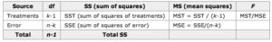ANOVA Calculation Table: This table summarizes the calculations necessary in an ANOVA for comparing multiple means.

Letting

$\text{x}_\text{ij}$

be the

$\text{j}$

th measurement in the

$\text{i}$

th sample (where

$\text{j}=1,2,⋯\text{n}$

), then:

Total

$$\text{SS}=\displaystyle\sum_{\text{i},\text{j}}(\text{x}_\text{ij}-\bar{\text{x}})^2=\sum{\text{x}_{\text{ij}}^2}-\frac{(\sum{\text{x}_{\text{ij}}})^2}{\text{n}}=\sum{\text{x}_{\text{ij}}^2}-\text{CM}$$

and the sum of the squares of the treatments is:

$\text{SST}=\sum{\text{n}_{\text{i}}(\bar{\text{x}}_{\text{i}}-\bar{\text{x}})^2}=\sum{\frac{\text{T}_{\text{i}}^2}{\text{n}_\text{i}}}-\text{CM}$

where

$\text{T}_\text{i}$

is the total of the observations in treatment

$\text{i}$

,

$\text{n}_\text{i}$

is the number of observations in sample

$\text{i}$

and

$\text{CM}$

is the correction of the mean:

$$\text{T}_\text{i}=\displaystyle\sum_{\text{j}}\text{x}_{\text{ij}}$$

$\text{CM}=\frac{(\sum{\text{x}_{\text{ij}}})^2}{\text{n}}$

The sum of squares of the error

$\text{SSE}$

is given by:

$\text{SSE}=\text{Total }\text{SS}-\text{SST}$

and

$\text{F}=\frac{\text{MST}}{\text{MSE}}$

.

Example

An example for the effect of breakfast on attention span (in minutes) for small children is summarized in the table below:

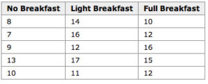Breakfast and Children's Attention Span: This table summarizes the effect of breakfast on attention span (in minutes) for small children.

The hypothesis test would be:

$\text{H}_0:\mu1=\mu2=\mu3$

versus:

$\text{H}_\text{a}:\mu1\neq\mu2 \text{ or }\mu2\neq\mu3\text{ or }\mu1\neq\mu3$

The solution to the test can be seen in the figure below:

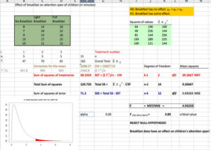Excel Solution: This image shows the solution to our ANOVA example performed in Excel.

The test statistic

$\text{F}$

is equal to 4.9326. The corresponding right-tail probability is 0.027, which means that if the significance level is 0.05, the test statistic would be in the rejection region, and therefore, the null-hypothesis would be rejected.

Hence, this indicates that the means are not equal (i.e., that sample values give sufficient evidence that not all means are the same). In terms of the example this means that breakfast (and its size) does have an effect on children's attention span.

Randomized Block Design

Block design is the arranging of experimental units into groups (blocks) that are similar to one another, to control for certain factors.

Learning Objectives

Reconstruct how the use of randomized block design is used to control the effects of nuisance factors.

Key Takeaways

KEY POINTS

• The basic concept of blocking is to create homogeneous blocks in which the nuisance factors are held constant, and the factor of interest is allowed to vary.
• Nuisance factors are those that may affect the measured result, but are not of primary interest.
• The general rule is: "Block what you can; randomize what you cannot." Blocking is used to remove the effects of a few of the most important nuisance variables. Randomization is then used to reduce the contaminating effects of the remaining nuisance variables.

KEY TERMS

• blocking: A schedule for conducting treatment combinations in an experimental study such that any effects on the experimental results due to a known change in raw materials, operators, machines, etc., become concentrated in the levels of the blocking variable.
• nuisance factors: Variables that may affect the measured results, but are not of primary interest.

What is Blocking?

In the statistical theory of the design of experiments, blocking is the arranging of experimental units in groups (blocks) that are similar to one another. Typically, a blocking factor is a source of variability that is not of primary interest to the experimenter. An example of a blocking factor might be the sex of a patient; by blocking on sex, this source of variability is controlled for, thus leading to greater accuracy.

Nuisance Factors

For randomized block designs, there is one factor or variable that is of primary interest. However, there are also several other nuisance factors. Nuisance factors are those that may affect the measured result, but are not of primary interest. For example, in applying a treatment, nuisance factors might be the specific operator who prepared the treatment, the time of day the experiment was run, and the room temperature. All experiments have nuisance factors. The experimenter will typically need to spend some time deciding which nuisance factors are important enough to keep track of or control, if possible, during the experiment.

When we can control nuisance factors, an important technique known as blocking can be used to reduce or eliminate the contribution to experimental error contributed by nuisance factors. The basic concept is to create homogeneous blocks in which the nuisance factors are held constant and the factor of interest is allowed to vary. Within blocks, it is possible to assess the effect of different levels of the factor of interest without having to worry about variations due to changes of the block factors, which are accounted for in the analysis.

The general rule is: "Block what you can; randomize what you cannot. " Blocking is used to remove the effects of a few of the most important nuisance variables. Randomization is then used to reduce the contaminating effects of the remaining nuisance variables.

Example

The progress of a particular type of cancer differs in women and men. A clinical experiment to compare two therapies for their cancer therefore treats gender as a blocking variable, as illustrated in . Two separate randomizations are done—one assigning the female subjects to the treatments and one assigning the male subjects. It is important to note that there is no randomization involved in making up the blocks. They are groups of subjects that differ in some way (gender in this case) that is apparent before the experiment begins.

Block Design: An example of a blocked design, where the blocking factor is gender.

Factorial Experiments: Two Factors

A full factorial experiment is an experiment whose design consists of two or more factors with discrete possible levels.

Learning Objectives

Outline the design of a factorial experiment, the corresponding notations, and the resulting analysis.

Key Takeaways

KEY POINTS

• A full factorial experiment allows the investigator to study the effect of each factor on the response variable, as well as the effects of interactions between factors on the response variable.
• The experimental units of a factorial experiment take on all possible combinations of the discrete levels across all such factors.
• To save space, the points in a two-level factorial experiment are often abbreviated with strings of plus and minus signs.

KEY TERMS

• level: The specific value of a factor in an experiment.
• factor: The explanatory, or independent, variable in an experiment.

A full factorial experiment is an experiment whose design consists of two or more factors, each with discrete possible values (or levels), and whose experimental units take on all possible combinations of these levels across all such factors. A full factorial design may also be called a fully crossed design. Such an experiment allows the investigator to study the effect of each factor on the response variable, as well as the effects of interactions between factors on the response variable.

For the vast majority of factorial experiments, each factor has only two levels. For example, with two factors each taking two levels, a factorial experiment would have four treatment combinations in total, and is usually called a

$2$

by

$2$

factorial design.

If the number of combinations in a full factorial design is too high to be logistically feasible, a fractional factorial design may be done, in which some of the possible combinations (usually at least half) are omitted.

Notation

To save space, the points in a two-level factorial experiment are often abbreviated with strings of plus and minus signs. The strings have as many symbols as factors, and their values dictate the level of each factor: conventionally, − for the first (or low) level, and + for the second (or high) level .

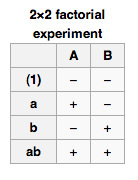Factorial Notation: This table shows the notation used for a

$2$

x

$2$

factorial experiment.

The factorial points can also be abbreviated by (

$1$

),

$\text{a}$

,

$\text{b}$

, and

$\text{ab}$

, where the presence of a letter indicates that the specified factor is at its high (or second) level and the absence of a letter indicates that the specified factor is at its low (or first) level (for example,

$\text{a}$

indicates that factor

$\text{A}$

is on its high setting, while all other factors are at their low (or first) setting). (

$1$

) is used to indicate that all factors are at their lowest (or first) values.

Analysis

A factorial experiment can be analyzed using ANOVA or regression analysis. It is relatively easy to estimate the main effect for a factor. To compute the main effect of a factor

$\text{A}$

, subtract the average response of all experimental runs for which

$\text{A}$

was at its low (or first) level from the average response of all experimental runs for which

$\text{A}$

was at its high (or second) level.

Other useful exploratory analysis tools for factorial experiments include main effects plots, interaction plots, and a normal probability plot of the estimated effects.

When the factors are continuous, two-level factorial designs assume that the effects are linear. If a quadratic effect is expected for a factor, a more complicated experiment should be used, such as a central composite design.

Example

The simplest factorial experiment contains two levels for each of two factors. Suppose an engineer wishes to study the total power used by each of two different motors,

$\text{A}$

and

$\text{B}$

, running at each of two different speeds,

$2000$

or

$3000$

RPM. The factorial experiment would consist of four experimental units: motor

$\text{A}$

at

$2000$

RPM, motor

$\text{B}$

at

$2000$

RPM, motor

$\text{A}$

at

$3000$

RPM, and motor

$\text{B}$

at

$3000$

RPM. Each combination of a single level selected from every factor is present once.

This experiment is an example of a

$2^2$

(or

$2$

by

$2$

) factorial experiment, so named because it considers two levels (the base) for each of two factors (the power or superscript), or

$(\text{number of levels})^{(\text{number of factors})}$

, producing

$2^2$

=

$4$

factorial points.

Designs can involve many independent variables. As a further example, the effects of three input variables can be evaluated in eight experimental conditions shown as the corners of a cube.

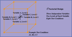Factorial Design: This figure is a sketch of a

$2$

by

$3$

factorial design.

This can be conducted with or without replication, depending on its intended purpose and available resources. It will provide the effects of the three independent variables on the dependent variable and possible interactions.

Licenses and Attributions

floraloven1978.blogspot.com

Source: https://www.coursehero.com/study-guides/boundless-statistics/comparing-more-than-two-means/

Share this post