Interpreting an Interaction Term for Continuous Vs Categorical Variables

The concept of a statistical interaction is one of those things that seems very abstract. Obtuse definitions, like this one from Wikipedia, don't help:

In statistics, an interaction may arise when considering the relationship among three or more variables, and describes a situation in which the simultaneous influence of two variables on a third is not additive. Most commonly, interactions are considered in the context of regression analyses.

First, we know this is true because we read it on the internet! Second, are you more confused now about interactions than you were before you read that definition?

If you're like me, you're wondering: What in the world is meant by "the relationship among three or more variables"? (As it turns out, the author of this definition is referring to an interaction between two predictor variables and their influence on the outcome variable.)

But, Wikipedia aside, statistical interaction isn't so bad once you really get it. (Stay with me here.)

Let's take a look at the interaction between two dummy coded categorical predictor variables.

The data set for our example is the 2014 General Social Survey conducted by the independent research organization NORC at the University of Chicago. The outcome variable for our linear regression will be "job prestige."  Job prestige is an index, ranked from 0 to 100, of 700 jobs put together by a group of sociologists. The higher the score, the more prestigious the job.

We'll regress job prestige on marital status (no/yes) and gender.

First question: Do married people have more prestigious jobs than non-married people?

(note: click any of the images in this post to see them larger)

The answer is yes. On average, married people have a job prestige score of 5.9 points higher than those not married.

Next question: Do men have jobs with higher prestige scores than women?

The answer is no. Our output tells us there is no difference between men and women as far as the prestige of their job. Men's average job prestige score is only .18 points higher than women, and this difference is not statistically significant.

But can we conclude that for all situations? Is it possible that the difference between job prestige scores for unmarried men and women is different than the difference between married men and women? Or will it be pretty much the same as the table above?

Here's where the concept of interaction comes in. We need to use an interaction term to determine that. With the interaction we'll generate predicted job prestige values for the following four groups: male-unmarried, female-unmarried, male-married and female-married.

Here are our results when we regression job prestige on marital status and gender and the interaction between married and male:

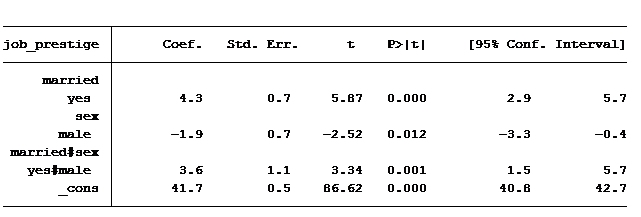
Everything is significant, but how in the world do we read this table? We are shown 4 values: married = 4.28, male = -1.86, married & male = 3.6 and the constant is 41.7. It helps to piece together the coefficients to create the predicted scores for the four groups mentioned above.

Let's start with the constant. It's in every regression table (unless we make the decision to exclude it). What exactly does it represent? The constant represents the predicted value when all variables are at their base case. In this situation our base case is married equals no and gender equals female (married = 0 and gender = 0).

So an unmarried woman has on average a predicted job prestige score of 41.7. An unmarried man's score is calculated by adding the coefficient for "male" to the constant (unmarried woman's score plus the value for being a male): 41.7-1.9 = 39.8.

To calculate a married woman's score we start with the constant (unmarried female) and add to it the value for being married: 41.7 + 4.3 = 46

How do we calculate a married man's score? Always start with the constant and then add to it any of the factors that belong to it. So we'll need to add to the constant the value of being married, of being male and also the extra value for being married and male: 41.7 + 4.3 – 1.9 + 3.6 = 47.7.

Notice that the difference in average job prestige score between unmarried women and unmarried men is 1.9 greater and the difference in average job prestige score between married women and married men is 1.7 less. The difference in those differences is  3.6 (1.9 – (-1.7), which is exactly the same as the coefficient of our interaction.

For those of you who use Stata, the simple way to calculate the predicted values for all four groups is to use the post-estimation command margins .

margins sex#married, cformat(%6.2f)

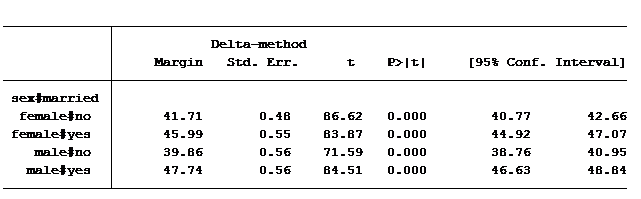
(These same means can be calculated using the lsmeans option in SAS's proc glm or using EMMeans in SPSS's Univariate GLM command).

If we had not used the interaction we would have concluded that there is no difference in the average job prestige score between men and women. By using the interaction, we found that there is a different relationship between gender and job prestige for unmarried compared to married people.

So that's it. Not so bad, right? Now go forth and analyze.

Jeff Meyer is a statistical consultant with The Analysis Factor, a stats mentor for Statistically Speaking membership, and a workshop instructor. Read more about Jeff here.

Interpreting Linear Regression Coefficients: A Walk Through Output

Learn the approach for understanding coefficients in that regression as we walk through output of a model that includes numerical and categorical predictors and an interaction.

floraloven1978.blogspot.com

Source: https://www.theanalysisfactor.com/interaction-dummy-variables-in-linear-regression/

Share this post